Linear mixed model in R

Data: Wheat Yield Trial

The data is originally from Stroup and Baenziger (1994) that is included as Wheat2 in nlme and as nin89 in asreml.

nin89 %>% ggplot(aes(Row, Column, fill=Rep)) + geom_tile() + ggtitle("Replicate Block")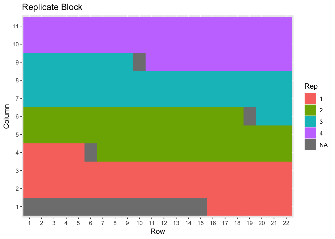

p <- nin89 %>% ggplot(aes(Row, Column, fill=Variety)) + geom_tile() + ggtitle("Variety Plot") 
ggplotly(p)

Fitting the linear mixed model in R

We want to the following model to the yield \(\boldsymbol{y}\): \[y=\boldsymbol{X}\boldsymbol{\tau} + \boldsymbol{Z}\boldsymbol{u} + \boldsymbol{e}\] where \(\boldsymbol{X}\) is the design matrix for the fixed variety effects \(\boldsymbol{\tau}\) and \(\boldsymbol{Z}\) is the design matrix for the random Block effect \(\boldsymbol{u}\) and \(\boldsymbol{e}\) is a vector of random error. We assume that \[\begin{bmatrix}\boldsymbol{u}\\ \boldsymbol{e} \end{bmatrix}\sim N\left(\begin{bmatrix}\boldsymbol{0}\\ \boldsymbol{0} \end{bmatrix}, \begin{bmatrix}\sigma^2_b\boldsymbol{I}_4 & \boldsymbol{0}\\ \boldsymbol{0} & \sigma^2\boldsymbol{\Sigma}_c \otimes\boldsymbol{\Sigma}_r \end{bmatrix}\right)\] where \(\sigma^2\boldsymbol{\Sigma}_c\) and \(\sigma^2\boldsymbol{\Sigma}_r\) are autoregressive process of order one for column and row direction, respectively.

We can fit the above model in asreml-R as below.

m0 <- asreml(yield ~ Variety, random=~Rep, rcov=~ar1(Column):ar1(Row), data=nin89, na.method.X="include", na.method.Y="include", aom=T)
asreml.variogram(x=1:nrow(nin89), z=m0$aom$R[,2]) %>% ggplot(aes(x, gamma)) + geom_point() + 
  theme_bw(base_size=16) + xlab("Unit Lag") + ylab("Empiricial Variogram for Stud. Cond. Residual")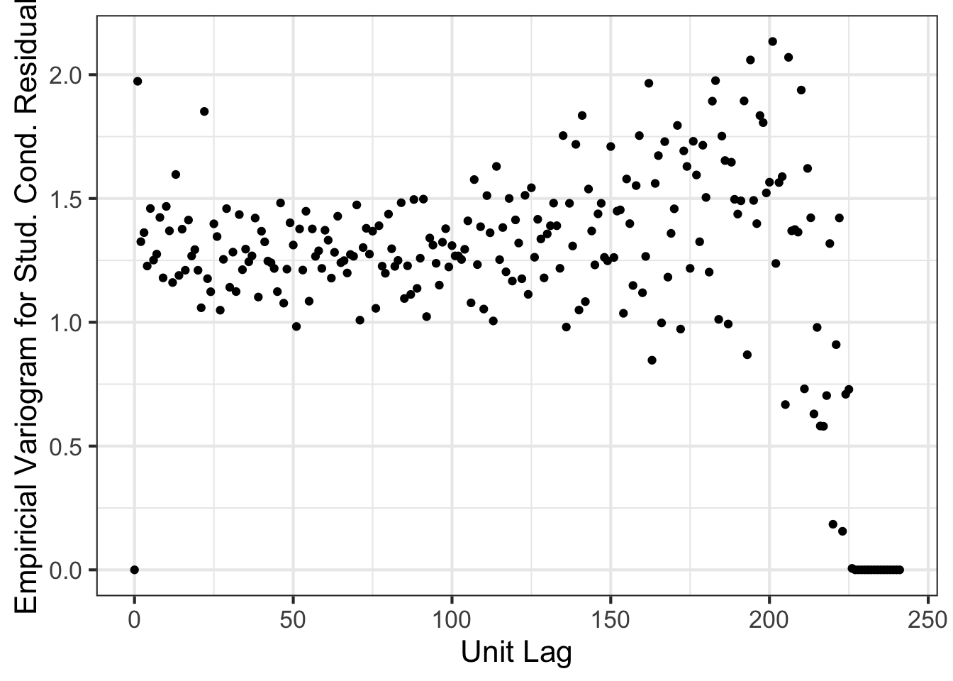

Most programs struggle to fit a multiplicative autoregressive structure as above. Is it important to fit such a structure though? Let’s assume instead that \({\rm var}(\boldsymbol{e}) = \sigma^2 \boldsymbol{I}_{242}\).

m1 <- asreml(yield ~ Variety, random=~Rep, rcov=~id(Column):id(Row), data=nin89, na.method.X="include", na.method.Y="include", aom=T)
asreml.variogram(x=1:nrow(nin89), z=m1$aom$R[,2]) %>% ggplot(aes(x, gamma)) + geom_point() + 
  theme_bw(base_size=16) + xlab("Unit Lag") + ylab("Empiricial Variogram for Stud. Cond. Residual")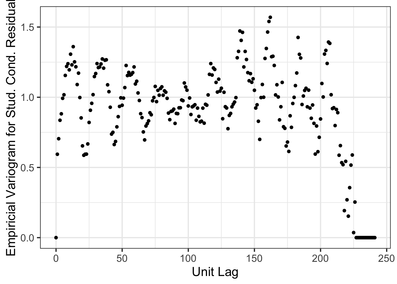

We can clearly see that there are some spatial trend that is not well captured by the second model.

A little about asreml-R

asreml-R fits a model by estimating the variance components using REML approach with the average information (AI) algorithm (Johnson and Thompson, 1995). This method was popularised and implemented in the stand-alone program ASreml (Gilmour et al., 1995) which is widely used, in particular by breeders. An interface for R was written based on the core algorithm in the stand-alone program, which we refer to as asreml-R (Butler et al., 2009). The asreml-R package is a powerful R-package to fit linear mixed models, with one huge advantage over competition is that, as far as I can see, it allows a lot of flexibility in the variance structures and more intuitive in its use.

The competing, alternative R-packages that fit the linear mixed models are nlme and lme4. Luis A. Apiolaza makes a comparison of these packages in his blog dated 2011/10/17. One downside is that asreml-R requires a license. This may be provided for free for educational or research purposes (details of which I am not aware of). Here is an attempt for the question dated 2011/11/01 to recreate the same analysis as asreml-R, although it appears spatial models (i.e. AR1\(\times\)AR1) cannot be easily recreated in open source packages. The dates are a bit old so perhaps the current situation may be different.